

Authorship analysis deals with the classification of texts into classes based on the stylistic choices of their authors. Beyond the author identification and author verification tasks where the style of individual authors is examined, author profiling distinguishes between classes of authors studying their sociology aspect, that is, how language is shared by people. This helps in identifying profiling aspects such as gender, age, native language, or personality type. Author profiling is a problem of growing importance in applications in forensics, security, and marketing. E.g., from a forensic linguistics perspective one would like being able to know the linguistic profile of the author of a harassing text message (language used by a certain type of people) and identify certain characteristics (language as evidence). Similarly, from a marketing viewpoint, companies may be interested in knowing, on the basis of the analysis of blogs and online product reviews, the demographics of people that like or dislike their products.
The authorship profiling task is often formulated as a classification problem, where a classifier is fed with a text and returns the corresponding gender or native language label. There are many machine learning methods that can be used in the classification task. We will be using the state of the art BERT (Bidirectional Encoder Representations from Transformers) which uses the base version with 12 layers.
Dataset:
• train_labels.csv: contains training ids (ID) and gender(label). It contains twitter posts from 3,100 authors and acts as the training data. You can download it from here
• test_labels.csv: contains the training ids(ID) and true gender(label) values. It acts as the test data. You can download it from here
Pre-processing:
Before creating the classifier, pre-processing the data and generating features is important to get rid of the irrelevant information and capturing the best features and certain trends.
Following are the pre-processing tasks done on the dataset:
- Using regular expressions, we removed the unwanted elements present in the tweets.
We removed all hyperlinks, emojis, and other non-alphabets form tweets. We have also removed the username which are starting from @, which do not have any semantics. - After removing the unwanted elements, we observed that there were leading white spaces in the tweets, so using ‘lstrip()’ removed the whitespaces as well.
- We stored all the textual data into the list, in which each element is the value of the tweets in the train dataset. Now, stemming and lemming is performed on the list to generate the root form of the inflected words of all the tweets.
- Next, we created the stopwords_list form NLTK corpus. Stopwords are those words that are extremely common and carry little lexical content. Stopwords should be removed as they are redundant and have less impact while natural language processing.
First, we check for the Graphics Processor, if it is available and find out which GPU we will be using for our task.
import tensorflow as tf

# Get the GPU device name.
device_name = tf.test.gpu_device_name()

# The device name should look like the following:
if device_name == '/device:GPU:0':
    print('Found GPU at: {}'.format(device_name))
else:
    raise SystemError('GPU device not found')
import torch

# If there's a GPU available...
if torch.cuda.is_available():

    # Tell PyTorch to use the GPU.
    device = torch.device("cuda")

    print('There are %d GPU(s) available.' % torch.cuda.device_count())

    print('We will use the GPU:', torch.cuda.get_device_name(0))

# If not...
else:
    print('No GPU available, using the CPU instead.')
    device = torch.device("cpu")
Then we load the above dataset into the Google Collab and perform the Pre-Processing Steps which are listed above.
After Pre-Processing we Tokenize the sentences using the bertTokenizer() which is included in the Transformers library. Tokenizer tokenizes each word in the sentence and assigns a number which is the token id.
Bert takes specific input in the form of CLS + sentence + SEP for each of the sentence, then uses padding to pad the empty characters in the sentence until Max Len is reached, then attention masks are used to identify which are the real tokens and which are the blank tokens used for padding.The MAX LEN can be is set to 64 as we can see that we don’t have any sentence beyond 64 characters and this length can be expanded up to 128.
# We'll borrow the `pad_sequences` utility function to do this.
from keras.preprocessing.sequence import pad_sequences

# Set the maximum sequence length.
# I've chosen 64 somewhat arbitrarily. It's slightly larger than the
# maximum training sentence length of 47...
MAX_LEN = 64

print('\nPadding/truncating all sentences to %d values...' % MAX_LEN)

print('\nPadding token: "{:}", ID: {:}'.format(tokenizer.pad_token, tokenizer.pad_token_id))

# Pad our input tokens with value 0.
# "post" indicates that we want to pad and truncate at the end of the sequence,
# as opposed to the beginning.
input_ids = pad_sequences(input_ids, maxlen=MAX_LEN, dtype="long",
                          value=0, truncating="post", padding="post")
Then the Training Validation is used where the training data is split into 90 and 10 percent respectively and then trained over 4 epochs trying to reduce the training loss and improve the accuracy on the training validation. Use the train_test_split from the sklearn library and convert the inputs and lables into torch tensors, which is the required datatype for our model.
# Create attention masks
attention_masks = []

# For each sentence...
for sent in input_ids:

    # Create the attention mask.
    #   - If a token ID is 0, then it's padding, set the mask to 0.
    #   - If a token ID is > 0, then it's a real token, set the mask to 1.
    att_mask = [int(token_id > 0) for token_id in sent]

    # Store the attention mask for this sentence.
    attention_masks.append(att_mask)

# Use train_test_split to split our data into train and validation sets for
# training
from sklearn.model_selection import train_test_split

# Use 90% for training and 10% for validation.
train_inputs, validation_inputs, train_labels, validation_labels = train_test_split(input_ids, labels,
                                                            random_state=2018, test_size=0.1)
# Do the same for the masks.
train_masks, validation_masks, _, _ = train_test_split(attention_masks, labels,
                                             random_state=2018, test_size=0.1)

# Convert all inputs and labels into torch tensors, the required datatype
# for our model.
train_inputs = torch.tensor(train_inputs)
validation_inputs = torch.tensor(validation_inputs)

train_labels = torch.tensor(train_labels)
validation_labels = torch.tensor(validation_labels)

train_masks = torch.tensor(train_masks)
validation_masks = torch.tensor(validation_masks)
The Data loader needs to know the batch size for training data, here we use the batch size as 32 we are fine tuning our BERT model. Now we, create Data Loader for the Training set with the Random Sampler and Data Loader for the Validation set with the sequential sampler. Then finally we create our model with the help of Transformers library and use BERT for Sequence Classification and build it according to our need and let pytorch run the model on the GPU.
from torch.utils.data import TensorDataset, DataLoader, RandomSampler, SequentialSampler

# The DataLoader needs to know our batch size for training, so we specify it
# here.
# For fine-tuning BERT on a specific task, the authors recommend a batch size of
# 16 or 32.

batch_size = 32

# Create the DataLoader for our training set.
train_data = TensorDataset(train_inputs, train_masks, train_labels)
train_sampler = RandomSampler(train_data)
train_dataloader = DataLoader(train_data, sampler=train_sampler, batch_size=batch_size)

# Create the DataLoader for our validation set.
validation_data = TensorDataset(validation_inputs, validation_masks, validation_labels)
validation_sampler = SequentialSampler(validation_data)
validation_dataloader = DataLoader(validation_data, sampler=validation_sampler, batch_size=batch_size)
from transformers import BertForSequenceClassification, AdamW, BertConfig

# Load BertForSequenceClassification, the pretrained BERT model with a single
# linear classification layer on top.
model = BertForSequenceClassification.from_pretrained(
    "bert-base-uncased", # Use the 12-layer BERT model, with an uncased vocab.
    num_labels = 2, # The number of output labels--2 for binary classification.
                    # You can increase this for multi-class tasks.
    output_attentions = False, # Whether the model returns attentions weights.
    output_hidden_states = False, # Whether the model returns all hidden-states.
)

# Tell pytorch to run this model on the GPU.
model.cuda()
Now that our model is created we begin by optimizing the model with the help of Adam Optimizer which is a very popular optimizer. We set the learning rate and epsilon values with weight decay fixed. And then begin to use the model on our training data. We define the number of epochs, steps and the accuracy function and then start the Training phase.
# Note: AdamW is a class from the huggingface library (as opposed to pytorch)
# I believe the 'W' stands for 'Weight Decay fix"
optimizer = AdamW(model.parameters(),
                  lr = 2e-5, # args.learning_rate - default is 5e-5, our notebook had 2e-5
                  eps = 1e-8 # args.adam_epsilon  - default is 1e-8.
                )
from transformers import get_linear_schedule_with_warmup

# Number of training epochs (authors recommend between 2 and 4)
epochs = 4

# Total number of training steps is number of batches * number of epochs.
total_steps = len(train_dataloader) * epochs

# Create the learning rate scheduler.
scheduler = get_linear_schedule_with_warmup(optimizer,
                                            num_warmup_steps = 0, # Default value in run_glue.py
                                            num_training_steps = total_steps)
Then Finally, we run the model with 4 epochs with each epoch almost lasting for 30 minutes. So after 2 hours of training and validation testing, we are able to see the Training loss decrease over the number of epochs. In order to see how much time is remaining, we print the batch and the time elapsed over it.
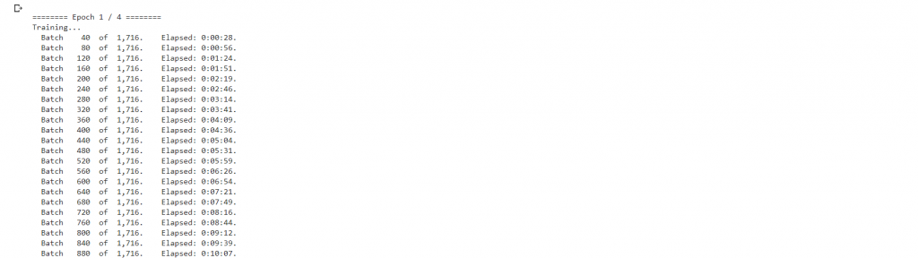
Put the model for training and it will take approximately 30 minutes for each epoch to train. Alternatively if you want to see the results fast, use sampling of the dataset. Sampling will reduce the time for training and will give results which are closer to actual results. I will explain the benefits of Sampling in another blog.
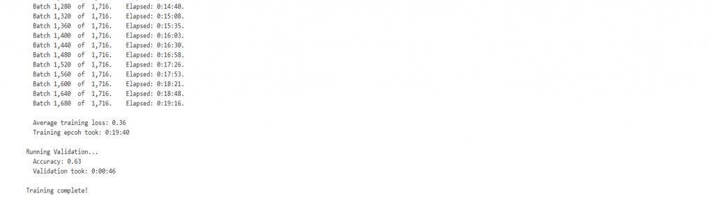
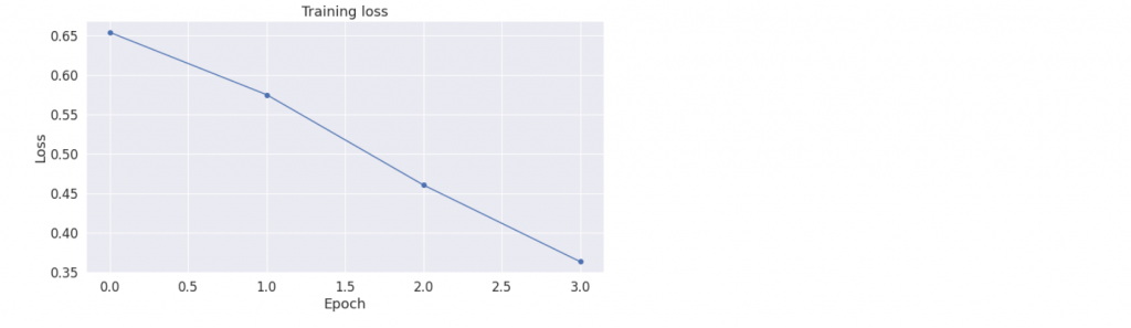
Visualize and observe the Training Loss over time and how it is decreasing with every epoch count. Here the Training Loss was almost 65 % in the first epoch and then reduced over time to 36 % by the end of last epoch. Accuracy may slightly differ but it is fine as that will depend on the training loss and it is not the final accuracy just the validation set accuracy.
Now we have finished our validation set testing and then we move onto the Test data. Note that validation set testing is a part of training dataset and not the Test data. Test Data should never be used while training the model. Now perform the pre-processing and all the above data transformation steps performed on the training data onto the test data. Now the format of the test data is similar to the train data. The code below will show the same process performed on the train data.
# Report the number of sentences.
print('Number of test sentences: {:,}\n'.format(df.shape[0]))

# Create sentence and label lists
sentences = df.sentence.values
labels = df.label.values
# Tokenize all of the sentences and map the tokens to thier word IDs.
input_ids = []
# For every sentence...
for sent in sentences:
    # `encode` will:
    #   (1) Tokenize the sentence.
    #   (2) Prepend the `[CLS]` token to the start.
    #   (3) Append the `[SEP]` token to the end.
    #   (4) Map tokens to their IDs.
    encoded_sent = tokenizer.encode(
                        sent,                      # Sentence to encode.
                        add_special_tokens = True, # Add '[CLS]' and '[SEP]'
                   )

    input_ids.append(encoded_sent)
# Pad our input tokens
input_ids = pad_sequences(input_ids, maxlen=MAX_LEN,
                          dtype="long", truncating="post", padding="post")
# Create attention masks
attention_masks = []
# Create a mask of 1s for each token followed by 0s for padding
for seq in input_ids:
  seq_mask = [float(i>0) for i in seq]
  attention_masks.append(seq_mask)
# Convert to tensors.
prediction_inputs = torch.tensor(input_ids)
prediction_masks = torch.tensor(attention_masks)
prediction_labels = torch.tensor(labels)
# Set the batch size.
batch_size = 32

# Create the DataLoader.
prediction_data = TensorDataset(prediction_inputs, prediction_masks, prediction_labels)
prediction_sampler = SequentialSampler(prediction_data)
prediction_dataloader = DataLoader(prediction_data, sampler=prediction_sampler, batch_size=batch_size)
Finally we predict the values on the test set. In our case this will be the gender of the authors which is fine tuned by our model. BERT is State of the Art (SOA) model and leaded by GPT 3 which has more than 175 billion parameters. the predictions are stored and then compared with the true gender of the authors to find out accuracy. In simple words, Accuracy is number of correctly predicted genders to the total number of genders.
# Prediction on test set

print('Predicting labels for {:,} test sentences...'.format(len(prediction_inputs)))

# Put model in evaluation mode
model.eval()

# Tracking variables
predictions , true_labels = [], []

# Predict
for batch in prediction_dataloader:
  # Add batch to GPU
  batch = tuple(t.to(device) for t in batch)

  # Unpack the inputs from our dataloader
  b_input_ids, b_input_mask, b_labels = batch

  # Telling the model not to compute or store gradients, saving memory and
  # speeding up prediction
  with torch.no_grad():
      # Forward pass, calculate logit predictions
      outputs = model(b_input_ids, token_type_ids=None,
                      attention_mask=b_input_mask)

  logits = outputs[0]

  # Move logits and labels to CPU
  logits = logits.detach().cpu().numpy()
  label_ids = b_labels.to('cpu').numpy()

  # Store predictions and true labels
  predictions.append(logits)
  true_labels.append(label_ids)

print('    DONE.')
Accuracy tells us whether a model is good model or not. But it may not always depend on Accuracy. For Classification problems we have Confusion Matrix, Precision, Recall and F1 Score which will help us in identifying whether a model is good model or not as sometimes there will overfitting and underfitting of the model, which should be avoided.
• true_labels.csv: contains training ids (ID) and gender(label). It contains twitter posts from 500 authors with their true Genders. You can use it to check the accuracy of your model and can download it from here
The Accuracy of our model is 79.8% which is pretty good as compared with SGDClassifier or RandomForest Classifier where the accuracy was just above 60%. The confusion matrix has displays 208 True Positives, 44 False Positives, 191 True Negatives and 57 False Negatives. The metrics of Precision, Recall and F1Score are displayed which can be calculated by,
• Precision = TP/TP+FP
• Recall = TP/TP+FN
• F1Score = 2*(Recall * Precision) / (Recall + Precision)
from sklearn.metrics import accuracy_score

y_true = btest['gender'].tolist()
y_pred = btest['bert_gender'].tolist()

print('The accuracy from the Bert classifier is,',accuracy_score(y_true, y_pred))

from sklearn import metrics
print("Some basic stastistical measures for this model are")
print(metrics.classification_report(y_true, y_pred))

print("The Confusion Matrix is")
print(metrics.confusion_matrix(y_true, y_pred))
If you would like to have access to the full code with comments of the above application please send me an email or contact me on LinkedIn and I will grant you the access to the code. It is 100% FREE!